Bayesian-Calibration of the Liquid-Drop Model
Overview
This exercise involves calibrating the Liquid Drop Model with a Bayesian approach and compare those results with a non-bayesian approach. The non-Bayesian approach I chose was scipy.optimize's curve_fit function, which uses non-linear least squares to fit a function to data. The Bayesian approach was implemented using the emcee package in Python, which uses a Markov Chain Monte Carlo (MCMC) method to sample from the posterior distribution of the model parameters. Rather than producing a single point estimate, this approach yields a full probability distribution for each coefficient, allowing us to quantify uncertainty in the parameter estimates. A uniform prior was assumed for each parameter, meaning no strong assumptions were made about their values before fitting to the data.
Problem Statement
The liquid-drop model is a nuclear model that is used to approximate the mass of an atomic nucleus from its number of protons and neutrons. It treats the nucleus as a drop of incompressible fluid of very high density, held together by the nuclear force. The model's formula is as follows:
where \(E_B\) is the binding energy, \(A\) is the total number of nucleons (mass number), \(Z\) us the number of protons (atom number), and \(a_V\), \(a_S\), \(a_C\), \(a_A\) are derived coefficients corresponding to the volumne energy, surface energy, coulomb energy, asymmetry energy, and pairing energy, respectively. The goal of this exercise is to fit the model to the data and find the energy coefficients with uncertainty. The data used is a list of several different nuclei with their mass number, atom number, and atomic mass listed.
Technical Approach
Key Components:
- Bayesian Optimization: Used Gaussian Process-based optimization to intelligently search the hyperparameter space.
- Hidden Markov Monte Carlo: Sampled from the posterior distributions of the model parameters.
Optimized Parameters:
- \(a_V\): Volume term
- \(a_S\): Surface term
- \(a_C\): Coulomb term
- \(a_A\): Asymmetry term
- \(\log(f)\): Term that accounts for any underestimated uncertainty in the model.
Results & Impact

Figure 1: Corner plot of posterior distributions of fitted coefficients.
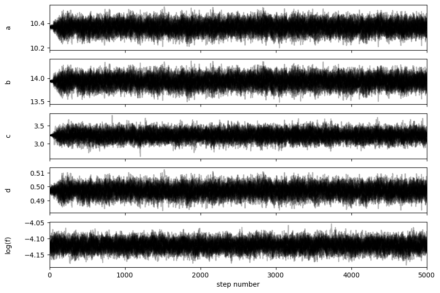
Figure 2: A walker trace plot that shows the evolution of each parameter across all walkers.
The corner plot above shows the posterior distributions for each of the five parameters: \(a\), \(b\), \(c\), \(d\), and \(\log(f)\). The diagonal histograms show the marginalized distribution for each parameter, while the off-diagonal panels show the joint distributions between parameter pairs, revealing any correlations.
The recovered parameter estimates with their 1\(\sigma\) uncertainties are:
Comparing these to commonly accepted literature values — \(a_V \approx 15.5\) MeV, \(a_S \approx 17.2\) MeV, \(a_C \approx 0.70\) MeV, and \(a_A \approx 23\) MeV — reveals notable discrepancies, particularly in \(a_C\) and \(a_A\). These differences are likely attributable to the subset of nuclei used for fitting: by restricting the dataset to heavier nuclei, the model is calibrated to a regime where certain terms contribute differently than across the full nuclear chart. The volume and surface coefficients \(a_V\) and \(a_S\) are also lower than literature values, which is consistent with fitting to a narrower mass range.
A strong positive correlation is visible between \(a\) and \(b\), as well as between \(b\) and \(d\), suggesting these coefficient pairs are not fully independent given the data. The \(\log(f)\) parameter, which accounts for any underestimated uncertainty in the model, converged to \(-4.121^{+0.014}_{-0.014}\), indicating the additional model error is small.